You will never think about buying UDFs ever again
Get access to high quality UDFs for free
Mathematical Methods UDFs
Calculus
Average Rate of Change (avgroc)
Function: Determines the average rate of change of a function
Syntax: avgroc(function, variable, lower, upper)
Example:
Average Value (avgval)
Function: Calculates the average value of a function
Syntax: avgval(function, variable, lower, upper)
Example:
Bound Area (boundarea)
Function: Determines the area bound by two graphs (if any) across their maximal domains
Syntax: boundarea(function1, function2, variable)
Example:
Bound Area with domain (boundaread)
Function: Determines the bound area between two functions in a restricted domain
Syntax: boundaread(function1, function2, variable, lower, upper)
Example:
Integral Solve (intsolve)
Function: Determines the answer for the integration multiple choice questions
Case 1: One integral given, find transformed integral
Syntax: intsolve({lower1,upper1, value1}, {transformations}, {lower2, upper2})
Example:
Case 2: Two integrals given, find untransformed integral
Syntax: intsolve({lower1, upper1, value1}, {lower2, upper2, value2}, {lower3, upper3})
Example:
Case 3: Two integrals given, find transformed integral
Syntax: intsolve({lower1, upper1, value1, lower2, upper2, value2}, {transformations}, {lower3, upper3})
Example:
Newton's Method (newtons)
Function: Estimates the root of a function using newton's method
Syntax: newtons(function, variable, x0, iterations)
Example:
Number of Roots (nroot)
Function: Determines the value(s) of a parameter required for a specified number of roots.
Syntax: nroot(polynomial, variable, parameter, number of roots)
Example:
Number of Stationary Points (nstp)
Function: Determines the value(s) of a parameter required for a specified number of stationary points.
Syntax: nstp(polynomial, variable, parameter, number of stationary points)
Example:
Number of Points of Inflection (npoi)
Function: Determines the value(s) of a parameter required for a specified number of points of inflection.
Syntax: npoi(polynomial, variable, parameter, number of points of inflection)
Example:
Points of Inflection (pois)
Function: Determines the points of inflection of a function
Syntax: pois(function, variable)
Example:
Sign Table (signtab)
Function: Uses a sign table to determine the stationary points of a function and their nature
Syntax: signtab(function, variable)
Example:
Stationary Points (stps)
Function: Determines the stationary points of a function
Syntax: stps(function, variable)
Example:
Tangent Solve (tangsolve)
Function: Determines the equation of the tangents to a function which pass through a specified point
Syntax: tangsolve(function, variable, x-coordinate, y-coordinate)
Example:
Trapezoid Approximation (trapapprox)
Function: Approximates an integral using the trapezoidal rule
Syntax: trapapprox(function, variable, lower, upper, number of trapezia)
Example:
Continuous Probability
Continuous Conditional Probability (ccondpr)
Function: Determines conditional probability for a continuous distribution
Case 1: Probability density function
Syntax: ccondpr(Probability Density Function, Lower Bound, Upper Bound, Condition 1, Condition 2)
Example:
Case 2: Normal Distribution
Syntax: ccondpr(Blank String, Mean, Standard Deviation, Condition 1, Condition 2)
Example:
Confidence Interval (confint)
Function: Determines a confidence interval as well as the z-score, margin of error and standard deviation
Syntax: confint(Sample Size,P_hat, . confidence)
Example:
Confidence Interval Solve (confintsolve)
Function: Determines the sample size, standard deviation or percentage confidence depending on the provided data
Syntax: confintsolve(Lower Bound, Upper Bound, Sample Size or Sample Standard Deviation or . Confidence)
Example:
Continuous Distribution Information (continfo)
Function: Determines the expected value, mean, variance, standard deviation of a continuous probability distribution
Syntax: continfo(function, variable, lower, upper)
Example:
Inverse Normal (invnormvals)
Function: Determines the left, right and centre possibilities for probability of a distribution
Syntax: invnormvals(mean, standard deviation, probability)
Example:
Normal Solve (normsolve)
Function: Determines the mean and standard deviation for lower and upper type questions
Case 1: Both Lower and Upper given
Syntax: normsolve(Lower, Probability of Lower, Upper, Probability of Upper)
Example:
Case 2: Lower and Mean given
Syntax: normsolve(Lower, Probability of Lower, Mean, Blank String)
Example:
Case 3: Lower and Standard Deviation given
Syntax: normsolve(Lower, Probability of Lower, Blank String, Standard Deviation)
Example:
Case 4: Upper and Mean given
Syntax: normsolve(Mean, Blank String, Upper, Probability of Upper)
Example:
Case 5: Upper and Standard Deviation given
Syntax: normsolve(Blank String, Standard Deviation, Upper, Probability of Upper)
Example:
Discrete Probability
Binomial Distribution Information (binominfo)
Function: Determines the expected value, variance, standard deviation, sample expected value, and sample standard deviation for a binomial distribution
Syntax: binominfo(Sample Size, Probability of Success)
Example:
Binomial Solve (binomsolve)
Function: Determines the number of trials required to achieve a certain probability
Syntax: binomsolve(outcome, probability of success, threshold value)
Example:
Discrete Conditional Probability (dcondpr)
Function: Determines conditional probability for a discrete distribution
Case 1: Binomial Distribution
Syntax: dcondpr(number of trials, probability of success, condition 1, condition 2)
Example:
Case 2: Discrete Probability Table
Syntax: dcondpr({List containing outcomes}, {List containing probabilities}, condition 1, condition 2)
Example:
Case 3: Probability Mass Function
Syntax: dcondpr({List containing outcomes}, PMF, condition 1, condition 2)
Example:
Hypergeometric Cumulative Probability Function (hypergeocdf)
Function: Determines the probability of selecting items without replacement, but over an interval of outcomes
Syntax: hypergeocdf(sample size, population size, number of successful items, lower bound, upper bound)
Example:
Hypergeometric Probability Density Function (hypergeopdf)
Function: Determines the probability of selecting items without replacement, but for specific outcomes
Syntax: hypergeopdf(sample size, population size, number of successful items, outcome)
Example:
Inverse Binomial (invbinomial)
Function: Determines the outcome required to achieve the probability
Syntax: invbinomial(number of trials, probability of success, known probability value)
Example:
Probability Table (prtable)
Function: Determines the mean, variance, standard deviation of a probability table
Syntax: prtable({outcomes}, {probabilities})
Example:
Sample Distribution Binomial (samplebinom)
Function: Determines the distribution for the sample proportion of a binomially distributed sample
Syntax: samplebinom(Sample Size, Probability of Success)
Example:
Sample Binomial Probability (samplebinompr)
Function: Determines the probability for the sample proportion for a binomially distributed sample
Syntax: samplebinompr(Sample Size, Probability of Success, Lower, Upper)
Example:
Sample Distribution Hypergeometric (samplehypergeo)
Function: Determines the distribution for the sample proportion of a hypergeometrically distributed sample
Syntax: samplehypergeo(Sample Size, Population Size, Number Successful)
Example:
Sample Hypergeometric probability (samplehyppr)
Function: Determines the probability for the sample proportion for a hypergeometrically distributed sample
Syntax: samplehyppr(Sample Size, Population Size, Number Successful, Lower, Upper)
Example:
Functions
Asymptotes (asymp)
Function: Determines the vertical and horizontal asymptotes of a function
Syntax: asymp(function, variable)
Example:
Composite Check (ccheck)
Function: Checks whether a composite function is valid, and the maximal domain required for the composite to be valid.
Syntax: ccheck(function 1, function 2)
Example:
Discriminant (discrim)
Function: Calculates the discriminant of an inputted quadratic expression
Syntax: discrim(quadratic Expr, variable)
Example:
Domain and Range (domrang)
Function: Determines the domain and range of a function
Syntax: domrang(function, variable)
Example:
Intercepts (intercepts)
Function: Finding the x and y intercepts of a function
Syntax: intercepts(function,variable)
Example:
Intersects (intersects)
Function: Determines the points of intersection of two functions across their maximal domains.
Syntax: intersects(function1,function2,variable)
Example:
Intersects with domain (intersectsd)
Function: Determines the points of intersection between two functions in a restricted domain
Syntax: intersectsd(function1, function2, variable, lower, upper)
Example:
Inverse Function (inverse)
Function: Determines the inverse of a function
Syntax: inverse(function, variable, x in domain of f)
Example:
Inverse Intersections (invints)
Function: Determines the values of a parameter, k, required for a function and its inverse function to have a certain number of intersections
Case 1: Square Root
Syntax: invints(function, number of intersections with inverse)
Example:
Case 2: Parabola
Syntax: invints(function, number of intersections with inverse) *You will be prompted to enter an initial condition
Example:
Case 3: Exponential
Syntax: invints(function, number of intersections with inverse)
Example:
Case 4: Logarithm
Syntax: invints(function, number of intersections with inverse)
Example:
Case 5: Hyperbola
Syntax: invints(function, number of intersections with inverse)
Example:
Case 6: Simple Cubic (Either 0 or 1 turning points)
Syntax: invints(function, number of intersections with inverse)
Example:
Case 7: Complicated Cubic (More than 1 turning point)
Syntax: invints(function, number of intersections with inverse) *You will be prompted to enter the domain
Example:
Angle Between Two Lines (lineang)
Function: Determines the angle between two lines in degrees (Assumes CAS in raidans mode)
Syntax: lineang(Line 1, Line 2, Variable)
Example:
Unique, None, Infinite Solution (linesolve)
Function: Determines when two linear equations will have an unique, none or infinitely many solutions. Note: Equations must be in the form: Ax + By = C , rather than Ax + By + C = 0
Syntax: linesolve(Equation1, Equation2)
Example:
Property Check (pcheck)
Function: Determines which function satisfies a specific property
Syntax: pcheck(function, variable, LHS, RHS)
Example:
Point Information (pointinfo)
Function: Determines the gradient, perpendicular gradient, line, x and y intercepts of a line, midpoint, distance
Syntax: pointinfo(x1, y1, x2, y2)
Example:
Polynomial Fit (polyfit)
Function: Determines the equation of a polynomial which passes through a set of points.
Syntax: polyfit({x1, y1, x2, y2, ...})
Example:
Transformations (transform)
Function: Determines the transformed function after applying certain transformations
Syntax: transform(function, {transformations})
Example:
Miscellaneous
Column Augment (ca)
Function: Converts answer into easily readable matrix form
Case 1: One Variable
Syntax: surfarea(Function, t, Lower Bound, Upper Bound)
Example:
Case 2: Multiple Variables (Up to 5)
Syntax: ca(Ans, {var1, var2,..., var5}
Example:
Domain Solve (dsolve)
Function: Solves equations in a restricted domain
Syntax: dsolve(Equation, Variable, Lower Bound, Upper Bound)
Example:
Graph Information (graphinfo)
Function: Determines the endpoints, x-intercepts, y-intercepts, stationary points, points of inflection of a function
Case 1: Restricted Domain
Syntax: graphinfo(Function, Variable, Lower Bound, Upper Bound)
Example:
Case 2: Across Maximal Domain
Syntax: graphinfo(Function, Variable, Blank String, Random Character)
Example:
Rewrite (rr)
Function: Gets the right hand side of an equation/answer
Syntax: rr(Equation/Answer)
Example:
Triganometric Solve (tsolve)
Function: Gives exact values of circular function equations (Ones which TiNspire cannot properly solve on its own)
Case 1: Trigonometric Equation
Syntax: tsolve(Equation, Variable, Lower Bound, Upper Bound)
Example:
Case 2: Trigonometric Inequality
Syntax: tsolve(Inequality, Variable, Lower Bound, Upper Bound)
Example:
Specialist Mathematics UDFs
Calculus
Arc Length (arclength)
Function: Determines the arc length for parametric curve
Case 1: Function
Syntax: arclength(Function, Variable, Lower Bound, Upper Bound)
Example:
Case 2: Parametric Equation
Syntax: arclength(Vector, Variable, Lower, Upper)
Example:
Bound Volume (boundvol)
Function: Determines the volume of the solid formed by the region(s) bound by two curves
Syntax: boundvol(Function 1, Function 2, Variable)
Example:
Bound Volume Domain (boundvold)
Function: Determines the volume of the solid formed by the region(s) bound by two curves in a restricted domain
Syntax: boundvold(Function 1, Function 2, Variable, Lower Bound, Upper Bound)
Example:
Euler's Method (eulers)
Function: Uses euler's method to estimate the solution to a differential equation
Syntax: eulers(Differential Equation, Independent Variable, x0, xn, y0, step-size)
Example:
Mixing Problems (mix)
Function: Determines the differential equation of the mixing problem
Syntax: mix() (You will be prompted for inputs)
Example:
Rational Function (rational)
Function: Determines holes, straight line asymptotes, and oblique asymptotes of a rational function.
Syntax: rational(numerator, denominator, variable)
Example:
Surface Area of Solid (surfarea)
Function: Determines the surface area of a solid of revolution
Case 1: Function of x rotated about x-axis
Syntax: surfarea(Function, Variable, Lower Bound, Upper Bound)
Example:
Case 2: Function of y rotated about y-axis
Syntax: surfarea(Function, Variable, Lower Bound, Upper Bound)
Example:
Case 3: Function of x rotated about y-axis
Syntax: surfarea(Function, y, x-lower, x-upper)
Example:
Case 4: Parametric Equation
Syntax: surfarea(Function, t, Lower Bound, Upper Bound)
Example:
Complex Numbers
De Moivre's Theorem (demoiv)
Function: Determines the solutions to roots of unity questions
Syntax: demoiv(Power , Number)
Example:
Circle Locus First Form (locicir1)
Function: Determines cartesian equation of circle loci in the form |z - a| = r
Syntax: locicir1(Point , Radius)
Example:
Circle Locus Second Form (locicir2)
Function: Determines cartesian equation of circle loci in the form |z - a| = k|z - b|
Syntax: locicir2(Point 1, Point 2, k)
Example:
Ellipse Locus (lociellp)
Function: Determines cartesian equation of ellipse loci
Syntax: lociellp(Point 1, Point 2, Length)
Example:
Hyperbola Locus (locihyp)
Function: Determines cartesian equation of hyperbola loci
Syntax: locihyp(Point 1, Point 2, Length)
Example:
Line Locus (lociline)
Function: Determines cartesian equation of line in the form |z - a| = |z - b|
Syntax: lociline(Point 1, Point 2)
Example:
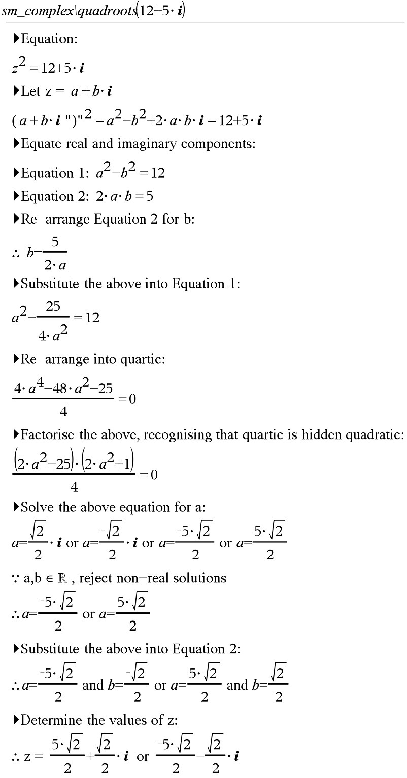
Quadratic Roots (quadroots)
Function: Determines quadratic roots of a complex number algebraically
Syntax: quadroots(Number)
Example:
Ray (ray)
Function: Determines the cartesian equation of a ray given a point and an angle
Syntax: ray(Point, Angle)
Example:
Kinematics
Collision Detector (collision)
Function: Determines whether two particles collide and where their paths intersect
Syntax: collision(Position Vector 1, Position Vector 2)
Example:
Projectile Motion (projm)
Function: Determines the accleration, velocity, position, max height, max displacement, return speed of a particle
Syntax: projm(Initial Position, Initial Velocity, Launch Angle, Initial Acceleration)
Example:
Constant Acceleration Equations (suvat)
Function: Enter 3 known values and 2 unknown variables, it will determine the unknowns
Syntax: suvat(s (displacement), u (initial velocity), v (final velocity), a (acceleration), t (time))
Example:
Vectors
Unit Vector Bisector (bisec)
Function: Determines the unit vector which bisects the angle between two vectors
Syntax: bisec(vector 1, vector 2)
Example:
Colinear (colin)
Function: Determines value(s) of a variable required for points to be collinear
Syntax: colin(Point 1, Point 2, Point 3)
Example:
Linear Dependence (lindep)
Function: Determines value(s) of a variable required for 3 vectors to be linearly dependent
Syntax: lindep(Vector 1, Vector 2, Vector 3)
Example:
Angle between Vectors (vecang)
Function: Determines the angle between the two inputted vectors.
Syntax: vecang(Vector1, Vector2)
Example:
Vector Projection (vproj)
Function: Determines vector, scalar resolute, & angle for two inputted vectors
Syntax: vproj(Vector 1, Vector 2)
Example:
Linear Algebra
Line Cartesian to Vector (car2vecline)
Function: Converts equation of line from cartesian form to vector form
Syntax: car2vecline(line Cartesian)
Example:
Plane Cartesian to Vector (car2vecplane)
Function: Converts equation of plane from cartesian form to vector form
Syntax: car2vecplane(Plane Cartesian)
Example:
Line Vector to Cartesian (vec2carline)
Function: Converts equation of line from vector form to cartesian form
Syntax: vec2carline(line Vector)
Example:
Plane Vector to Cartesian (vec2carplane)
Function: Converts equation of plane from vector form to cartesian form
Syntax: vec2carplane(Plane Vector)
Example:
Minimum Distance between 2 lines (dist2l)
Function: Determines minimum distance between two lines
Syntax: dist2l(Line Vector 1, Line Vector 2)
Example:
Minimum Distance between 2 planes (dist2pl)
Function: Determines minimum distance between two planes
Syntax: dist2pl(Plane Cartesian 1, Plane Cartesian 2)
Example:
Minimum Distance between line and plane (distlpl)
Function: Determines the minimum distance between a plane and line
Syntax: distlpl(Line Vector, Plane Cartesian)
Example:
Minimum Distance between line and point (distlp)
Function: Determines minimum distance between a line and point
Syntax: distlp(Line Vector, Point)
Example:
Minimum Distance between plane and point (distplp)
Function: Determines minimum distance between a plane and point
Syntax: distlp(Plane Equation, Point)
Example:
Intersection between 2 lines (ints2l)
Function: Determines the point of intersection & angle between two lines
Syntax: ints2l(Line Vector 1, Line Vector 2)
Example:
Intersection between 2 planes (ints2pl)
Function: Determines the line of intersection & angle between two planes
Syntax: ints2pl(Plane Cartesian 1, Plane Cartesian 2)
Example:
Intersection between plane and line (intslpl)
Function: Determines the point of intersection & angle between line and plane
Syntax: intslpl(Line Vector, Plane Cartesian)
Example:
Create line with 2 points (line2p)
Function: Determines the equation of a line given two points
Syntax: line2p(Point 1, Point 2)
Example:
Create line with direction vector and point (linedp)
Function: Determines the equation of a line given a direction vector and point
Syntax: linedp(Direction Vector, Point)
Example:
Create plane with 3 points (plane3p)
Function: Determines the equation of a plane given three points
Syntax: plane3p(Point 1, Point 2, Point 3)
Example:
Create plane with normal and point (planenp)
Function: Determines the equation of a plane given a normal vector and a point
Syntax: planenp(Normal Vector, Point)
Example:
Plane formed by intersecting lines (planeintl)
Function: Determines the equation of the plane formed by two intersecting lines
Syntax: planeintl(Line Vector 1, Line Vector 2)
Example:
Probability
Sample Mean Confidence Interval (confint)
Function: Determines the confidence interval for the sample mean
Syntax: confint(Sample Mean, Population Standard Deviation, Sample Size, . confidence)
Example:
Hypothesis Testing (hyptest)
Function: Determines whether the null hypothesis should be rejected by calculating p-values
Syntax: hyptest() (You will be prompted for inputs)
Example:
Probability of Error (prerror)
Function: Determines the probability of Type I and Type II errors occuring
Syntax: prerror() (You will be prompted for inputs)
Example:
p-value (pval)
Function: Determines the p-value of a hypothesis test
Syntax: pval() (You will be prompted for inputs)
Example:
Download
UDF Files:
Instructions on how to install the UDFs are available in Contact Us under "How do I install the UDFs?"
Note: Latest version is v3.1 for SM and v3.2 for MM. Please ensure that the version you install is up to date. Important: Due to limited time the new UDFs have not been extensively tested.
Latest Changes (v2.1 - v3.2)
Note: MM3&4 UDFs are intended for MM3&4, inputting SM3&4 functions may result in unexpected behaviour
Added new UDFs sm_calc\para_tangnorm, sm_calc\para_2nd_deriv, sm_calc\para_closep, sm_comp\segment, sm_calc\conic, mm_misc\triginfo, mm_func\bisec
Added warnings to new UDFs, and UDFs with bugs.
Fixed working out for sm_pr\confint and sm_calc\para_2nd_deriv, accidentally duplicated values (oops)
Bug fix to mm_calc\boundarea fixed issue where g(x) being greater than f(x) gave weird value
Bug fixes to sm_linalg\intslpl and sm_linalg\ints2pl (fixed issues when letting z = t gave weird solution)
Bug fix to sm_linalg\dist2l (fixed parallel line detection)
Bug fix to sm_kin\suvat and sm_pr\prerror (fixed working out so it formated correctly)
Added working out to sm_linalg\ints2pl
Added E(X), Var(X), Sd(X) to mm_dpr/samplebinom and mm_dpr/samplehypergeo
Made sm_linalg\ints UDFs find acute angle, as that's what questions usually ask for
UDF Guides:
Mathematical Methods UDF Guide
Specialist Mathematics UDF Guide
Note: The latest version is v3.1 for MM and v3.0 for SM Please ensure that the version you install is up to date.
Version Updates & Mailing List
New version v3: Added some extra requested UDFs. However, due to limited time the new UDFs have not been extensively tested.
Join our mailing list so you don't miss the latest updates :D sign up here
Program Bugs:
While the vast majority of the programs work fine, it's difficult for us to determine every single bug.
If you encounter any issues or difficulties, please contact us and we will try to help you out.
Bugs Unresolved:
Inverse intersections (invints) sometimes does not give accurate included/excluded values due to CAS approximation. Please make sure to verify the results graphically
nroots, nstps, npois don't work for non-polynomial functions, documentation has been updated to reflect this.
Trig Solve (tsolve) may provide inaccurate inqualities if a function in the equation has asymptotes.
Continous Information (continfo) sometimes may provide a weird (obviously wrong) answer for median sometimes idk why ... but then it works again if you reset CAS ???
Domain and Range function does not handle parameters well
Domain and Range may give inaccurate results if the domain is not restricted for complicated functions.
Domain and Range function does not handle rational functions well. Beware of auto-simplification.
Domain and Range function may round undefined endpoints into defined endpoints.